Take a single image#

Learn how to generate a single image.

Imports#

import numpy as np

import synpivimage

Set up the synthetic PIV components#

A synthetic PIV setup consists of

laser and
camera.

Let’s set up both components. If you need explanation for the parameters, please visit the documentation for laser and camera respectively.

We will use some standard parameters and choose a small image/sensor of 16x16 pixels:

cam = synpivimage.Camera(
    nx=16,
    ny=16,
    bit_depth=16,
    qe=1,
    sensitivity=1,
    baseline_noise=50,
    dark_noise=10,
    shot_noise=False,
    fill_ratio_x=1.0,
    fill_ratio_y=1.0,
    particle_image_diameter=2,
    seed=100
)

laser = synpivimage.Laser(
    width=0.25,
    shape_factor=2
)

Position particles#

Next, we need to define the position and size of the particles within the sensor plane.

By intention, we create particles outside the camera FOV, which are coordinates below 0 or larger than cam.nx or cam.ny. By taking the image later, the algorithm will flag particles, that are not illuminated.

n = 100
particles = synpivimage.Particles(
    x=np.random.uniform(-5, cam.nx+4, n),
    y=np.random.uniform(-5, cam.ny+4, n),
    z=np.zeros(n),
    size=np.ones(n)*2.5
)

Take the image#

To take the image, call take_image and pass the above components. You need to define the theoretical particle count of an image particle located at z=0.

img, part = synpivimage.take_image(
    laser,
    cam,
    particles,
    particle_peak_count=1000)

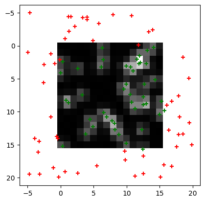
Let’s plot the image. Not all particles are illuminated. We will mark the illuminated ones green in the plot below. All illuminated (active) particles can be accessed using the flag via the property active:

import matplotlib.pyplot as plt

plt.imshow(img, cmap='gray')
plt.scatter(part.x[part.active],
            part.y[part.active],
            marker='+', color='g')
plt.scatter(part.x[~part.active],
            part.y[~part.active],
            marker='+', color='r')

<matplotlib.collections.PathCollection at 0x7f7e02db5fd0>

../_images/b64ec8f4479eb32a1faf1e243ab06a87a4dbcb98526aa931c44aab3e87c185f8.png

Read data#

The image can be read with cv2. The settings and particles can be read with synpivimage. Note, that the latter is stored as json-ld files, which allow anyone (human or machine) to read the data. The keys in the json document are put into context. More on this here.

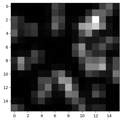
Read image#

To read the image data if stored as tif file, just use the open-cv package:

import cv2

img_loaded = cv2.imread('single_img/imgs/img_000000.tif', -1)
plt.imshow(img_loaded, cmap='gray')

<matplotlib.image.AxesImage at 0x7f7dfce1ceb0>

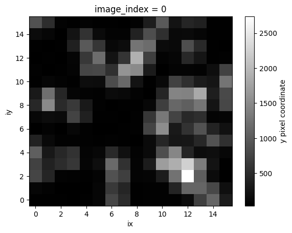
../_images/e65ce6c0e2284295ceb1a7ab8e0d2b1fe7c7f25866fb44f8f96bcd38e1eabab6.png

If data is stored in the HDF5 file, use h5py or h5tbx:

with h5tbx.File('single_img.hdf') as h5:
    imgAloaded = h5.images.img_A[()]
imgAloaded.plot(cmap='gray')

<matplotlib.collections.QuadMesh at 0x7f7dfcd7b850>

../_images/e512fd27d46f3362e0a234943ea53b3ea33bf5f58504d546e6f10eb947fa5be8.png

Read the setup#

The setup can be stored in JSON files (actually JSON-LD files, but the suffix is .json). If you wrote data to HDF5, then simply read the datasets “camera” and “laser” with their attribute.

In the following we will learn how to extract the data from the JSON-LD files using ontolutils

loaded_laser = synpivimage.Laser.load_jsonld('single_img/laser.json')
loaded_camera = synpivimage.Camera.load_jsonld('single_img/camera.json')

Experts: If you want to know how it is done, the following parts will show, what is going on behind load_jsonld:

In the background the rdflib library is used query the json-ld file with SPARQL. The library ontolutils further helps us with that and returns a dictionary for the type of thing we are looking for. For the laser, we are searching for types “pivmeta:LaserModel”:

import ontolutils

query_dict = ontolutils.dquery(
    'pivmeta:LaserModel',
    'single_img/laser.json',
    context={'pivmeta': 'https://matthiasprobst.github.io/pivmeta#'}
)

for p in query_dict[0]['hasParameter']:
    print(f"{p['label']:14s}: {p['hasNumericalValue']} (std name: {p['hasStandardName']})")

width         : 0.25 (std name: https://matthiasprobst.github.io/pivmeta#model_laser_sheet_thickness)
shape_factor  : 2 (std name: https://matthiasprobst.github.io/pivmeta#model_laser_sheet_shape_factor)

Note: Theoretically, there might be many lasers stored in the JSON file, this is why we get a list of dictionaries!

More useful than the above is retrieving the parameters as a dictionaries with the label as key (the label turns out to be exactly the object attributes of our components).

params = {p['label']: p.get('hasNumericalValue', p.get('hasStringValue', None)) for p in query_dict[0]['hasParameter']}
params

{'width': '0.25', 'shape_factor': '2'}

In the next step we can pass this to out component, in this case the laser:

synpivimage.Laser(**params)

Laser(shape_factor=2, width=0.25)

Comment on noise level#

If the dark noise is too high, the particle intensity and therefore its contribution to the cross correlation is considered to be indistinguishable from the noise. To illustrate, we regenerate the image from the beginning, now with too much dark noise:

cam.baseline_noise=100
cam.dark_noise=500
cam.shot_noise=False

img, part = synpivimage.take_image(
    laser,
    cam,
    particles,
    particle_peak_count=1000)

All particles are marked red. The gaussian noise image next to it shows that individual particles are barely identifiable.

fig, axs = plt.subplots(1, 2)
axs[0].imshow(img, cmap='gray', vmin=0, vmax=1500)
axs[0].scatter(part.x[part.active],
            part.y[part.active],
            marker='+', color='g')
axs[0].scatter(part.x[~part.active],
            part.y[~part.active],
            marker='+', color='r', alpha=0.25)

axs[1].set_title('Gaussian noise')
gnoise = np.random.normal(loc=cam.baseline_noise, scale=cam.dark_noise, size=(cam.ny, cam.nx))
gnoise[gnoise<0] = 0
axs[1].imshow(gnoise, cmap='gray', vmin=0, vmax=1500)
axs[1].set_xlim(axs[0].get_xlim())
axs[1].set_ylim(axs[0].get_ylim())

(21.177435506256714, -6.213366444905123)

../_images/9f5f9a04b6360068afbe4873cb829e69d7ab0a3a4dcfae87b44e51225ce7bdf6.png

Take a single image

Contents