Laser modelling#
The laser is modeled as outlined in “Particle Image Velocimetry: A Practical Guide” by Raffel et al.-
The laser width definition is a difficult parameter. Per definition, the laser beam shape is based on a Gaussian distribution with a shape factor (shape factor of 1 (Raffel et al. claims that it must be equal to 2, but this is not correct!) is a Gaussian profile, larger values will result in more top-hat shaped beams). The laser width \(\Delta Z0\) is where the (normalized) intensity drops to \(-1/\sqrt{2\pi} \approx 0.67\):
\begin{equation} I_0(Z) = q \cdot exp\left[ -\frac{1}{\sqrt{(2\pi)}} \left( \frac{2 Z^2}{\Delta Z_0^2} \right)^s \right] \end{equation}
The laser width is \(\Delta Z\) and the shape factor is \(s\). However, this is not the physical width! Why? Let’s build a
import numpy as np
import matplotlib.pyplot as plt

import synpivimage
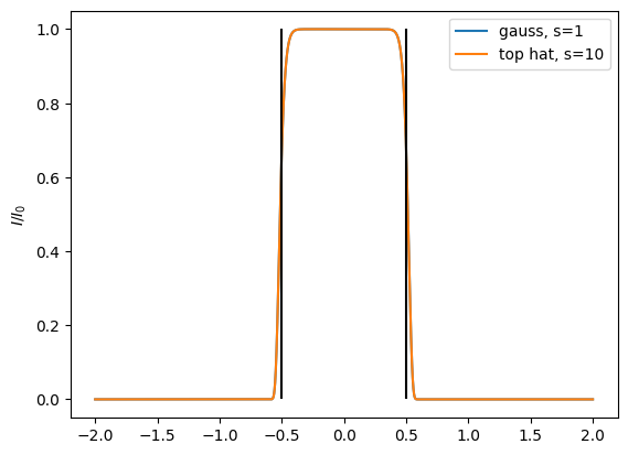
Gaussian vs. top-hat laser sheet profile#
Shape factor \(s\)=1 is a Gaussian laser sheet profile. To get a top-hat-like profile, use larger values, e.g. \(s=10\) or higher. In the below example, both sheets have a width of \(\Delta Z=1\), but note its definition!
z = np.linspace(-2, 2, 10000)
gauss_laser = synpivimage.Laser(
    width=1,
    shape_factor=1
)
tophat_laser = synpivimage.Laser(
    width=1,
    shape_factor=10
)
Position particles
many_particles = synpivimage.Particles(
    x=np.ones_like(z),
    y=np.ones_like(z),
    z=z,
    size=np.ones_like(z)
)
gauss_iluminated_particles = gauss_laser.illuminate(many_particles)
tophat_iluminated_particles = tophat_laser.illuminate(many_particles)
import matplotlib.pyplot as plt
Notice how both laser beam profiles will intersect the same intensity at \(I/I_0=0.67\)
plt.plot(z, gauss_iluminated_particles.irrad_photons, label='gauss, s=1')
plt.plot(z, tophat_iluminated_particles.irrad_photons, label='top hat, s=10')
plt.vlines(-gauss_laser.width/2, 0, 1, color='k')
plt.vlines(gauss_laser.width/2, 0, 1, color='k')
plt.ylabel('$I/I_0$')
plt.legend()
<matplotlib.legend.Legend at 0x7f2d22e0c8e0>
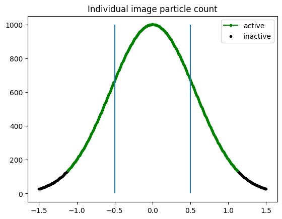
Whether or not a particle will be illuminated (also outside \(\Delta Z_0\)) depends on the noise level. With no noise, the limit is set to \(\exp(-2)\):
cam = synpivimage.Camera(
    nx=16,
    ny=16,
    bit_depth=16,
    qe=1,
    sensitivity=1,
    baseline_noise=0,
    dark_noise=0,
    shot_noise=False,
    fill_ratio_x=1.0,
    fill_ratio_y=1.0,
    particle_image_diameter=1.0
)
n = 400
many_particles = synpivimage.Particles(
    x=np.ones(n)*cam.nx//2,
    y=np.ones(n)*cam.ny//2,
    z=np.linspace(-3*gauss_laser.width / 2, 3*gauss_laser.width/2, n),
    size=np.ones(n)*2
)
imgOne, partOne = synpivimage.take_image(gauss_laser, cam, many_particles, particle_peak_count=1000)
plt.plot(partOne.z[partOne.active], partOne.max_image_photons[partOne.active], marker='.', color='g', label='active')
plt.scatter(partOne.z[~partOne.active], partOne.max_image_photons[~partOne.active], marker='.', color='k', label='inactive')
plt.title('Individual image particle count')
plt.vlines(-gauss_laser.width/2, 0, 1000)
plt.vlines(gauss_laser.width/2, 0, 1000)
plt.legend()
<matplotlib.legend.Legend at 0x7f2d1b2b6790>
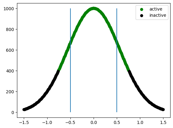
Influence of the noise level to the effective laser width#
If the Gaussian noise (dark_noise) is larger than a particle than it cannot be seen, hence this defines the laser width:
laser = synpivimage.Laser(
    width=1.0,
    shape_factor=1
)

cam = synpivimage.Camera(
    nx=16,
    ny=16,
    bit_depth=16,
    qe=1,
    sensitivity=1,
    baseline_noise=200,
    dark_noise=100,
    shot_noise=False,
    fill_ratio_x=1.0,
    fill_ratio_y=1.0,
    particle_image_diameter=1.0
)

many_particles.reset()
imgOne, partOne = synpivimage.take_image(laser, cam, many_particles, particle_peak_count=1000)


plt.scatter(partOne.z[partOne.active], partOne.max_image_photons[partOne.active], color='g', label='active')
plt.scatter(partOne.z[~partOne.active], partOne.max_image_photons[~partOne.active], color='k', label='inactive')
# plt.scatter(partOne.z[partOne.out_of_plane], partOne.max_image_photons[partOne.out_of_plane], color='y', label='inactive')
plt.vlines(-laser.width/2, 0, 1000)
plt.vlines(laser.width/2, 0, 1000)
plt.legend()
<matplotlib.legend.Legend at 0x7f2d1b1ec1c0>
one_particle = synpivimage.Particles(
x=[8, ],
y=[8, ],
z=[0, ],
size=[2, ]
)
from scipy.fft import rfft2, irfft2, fftshift
def compute_fft_xcorr(imgA, imgB):
"""Computes the cross-correlation of two images using the Fourier method."""
f2a = np.conj(rfft2(imgA))
f2b = rfft2(imgB)
return fftshift(irfft2(f2a * f2b).real, axes=(-2, -1))
def get_integer_peak(corr):
corr = np.asarray(corr)
ind = corr.ravel().argmax(-1)
peaks = np.array(np.unravel_index(ind, corr.shape[-2:]))
peaks = np.vstack((peaks[0], peaks[1])).T
index_list = [(i, v[0], v[1]) for i, v in enumerate(peaks)]
# peaks_max = np.nanmax(corr, axis=(-2, -1))
# np.array(index_list), np.array(peaks_max)
iy, ix = index_list[0][2], index_list[0][1]
return iy, ix
def gauss3pt(arr):
"""assuming highest peak is at the center of the array"""
assert arr.shape == (3, 3), f'Wrong shape {arr.shape}'
cl = arr[1, 0]
cc = arr[1, 1]
cr = arr[1, 2]
cu = arr[2, 1]
cd = arr[0, 1]
nom1 = np.log(cl) - np.log(cr)
den1 = 2 * np.log(cl) - 4 * np.log(cc) + 2 * np.log(cr)
nom2 = np.log(cd) - np.log(cu)
den2 = 2 * np.log(cd) - 4 * np.log(cc) + 2 * np.log(cu)
subp_peak_position = (
1 + np.divide(nom2, den2, out=np.zeros(1), where=(den2 != 0.0))[0],
1 + np.divide(nom1, den1, out=np.zeros(1), where=(den1 != 0.0))[0]
)
return subp_peak_position
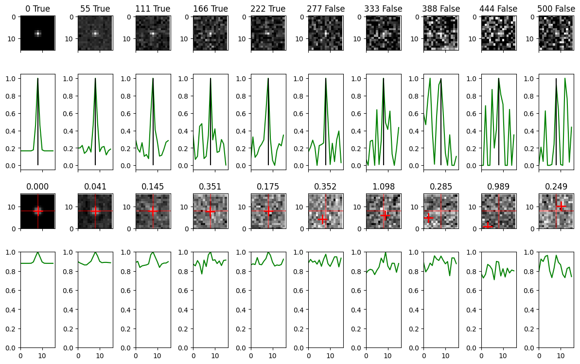
N = 10
fig, axs = plt.subplots(4, N, tight_layout=True, sharex=True,
figsize=(12, 8))
cam.particle_image_diameter = 2.5
for ii, dark_noise in enumerate(np.linspace(0, 500, N, dtype=int)):
cam.dark_noise = dark_noise
A, partA = synpivimage.take_image(laser, cam, one_particle, particle_peak_count=1000)
B, partB = synpivimage.take_image(laser, cam, one_particle, particle_peak_count=1000)
ny, nx = A.shape
axs[0][ii].set_title(str(dark_noise)+' '+str(partA.active[0]))
axs[0][ii].imshow(A, cmap='gray')
axs[1][ii].plot(A[8, :]/A[8, :].max(), color='g')
# axs[1][ii].plot(imgOne[:, 8]/imgOne[:, 8].max(), color='r')
axs[1][ii].vlines(8, 0, 1, color='k')
# compute auto correlation
auto_corr = compute_fft_xcorr(A[:], B[:])
j, i = get_integer_peak(auto_corr)
# get peak position
if j == 0:
j = 1
elif j == ny:
j = ny - 3
elif j == ny-1:
j = ny - 2
if i == 0:
i = 1
elif i == nx:
i = nx - 3
elif i == nx-1:
i = nx - 2
j0, i0 = gauss3pt(auto_corr[j-1:j+2, i-1:i+2])
dist = np.sqrt((j0-1)**2+(i0-1)**2)
# if i==0:
corr_norm = auto_corr.max()
axs[2][ii].imshow(auto_corr/corr_norm, cmap='gray')
axs[2][ii].vlines(8, 0, 16, color='r', alpha=0.5)
axs[2][ii].hlines(8, 0, 16, color='r', alpha=0.5)
axs[2][ii].scatter(i0+i-1, j0+j-1, marker='+', color='r', s=200, linewidths=2)
axs[2][ii].set_title(f'{dist:.3f}')
axs[2][ii].set_xlim([0, 16])
axs[2][ii].set_ylim([0, 16])
axs[3][ii].plot(auto_corr[8, :]/corr_norm, color='g')
axs[3][ii].set_ylim([0, 1])
# axs[3][i].plot(auto_corr[:, 8]/corr_norm, color='r')
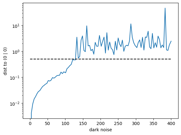
Find a noise level at which the autocorrelation shows no detectable peak#
N = 100
M = 100
dists = np.zeros(shape=(N, M))
for ii, dark_noise in enumerate(np.linspace(0, 400, N, dtype=int)):
    for m in range(M):
        cam.dark_noise = dark_noise
        A, partA = synpivimage.take_image(laser, cam, one_particle, particle_peak_count=1000)
        B, partB = synpivimage.take_image(laser, cam, one_particle, particle_peak_count=1000)

        auto_corr = compute_fft_xcorr(A[:], B[:])

        j, i = get_integer_peak(auto_corr)

        # get peak position
        if j == 0:
            j = 1
        elif j == ny:
            j = ny - 3
        elif j == ny-1:
            j = ny - 2

        if i == 0:
            i = 1
        elif i == nx:
            i = nx - 3
        elif i == nx-1:
            i = nx - 2

        j0, i0 = gauss3pt(auto_corr[j-1:j+2, i-1:i+2])
        dist = np.sqrt((j0-1)**2+(i0-1)**2)

        dists[ii][m] = dist
means = dists.mean(axis=1)
stds = dists.std(axis=1)
# plt.errorbar(x=np.linspace(0, 1000, N, dtype=int), y=means, yerr=stds)
plt.plot(np.linspace(0, 400, N, dtype=int), means)
plt.hlines(0.5, 0, 400, color='k', linestyle='--')
plt.xlabel('dark noise')
plt.ylabel('dist to (0 | 0)')
plt.yscale('log')